2.2 Transport
2.2.1 Roads Surface - Sealed/Unsealed
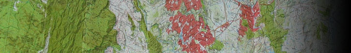
2.2.1.1 Example 1
| |
| Location of Example: |
152°43'28" East, 25°27'32" South |
| Distinctive Characteristics: |
- In Figure 2.2.1.1a the grey colour depicts the sealed road with evidence of white road markings compared with the light brown/yellow/white colour of the unsealed roads.
- In Figure 2.2.1.1b the blue/grey signature depicts the sealed road compared with the lighter yellow/white/blue signature that represents the unsealed roads.
|
| Regional Considerations: |
- In Peri-Urban areas roads frequently change from sealed to unsealed.
|
| Figure: 2.2.1.1 Representation of Sealed Roads and Unsealed Roads. |


[back to top]
2.2.1.2 Example 2
| |
| Location of Example: |
152°54'58" East, 25°25'10" South |
| Distinctive Characteristics: |
- In Figure 2.2.1.2a the grey colour depicts the sealed road compared with the light brown/white colour of the unsealed road.
- In Figure 2.2.1.2b the dark grey signature depicts the sealed road compared with the light grey/yellow/white signature that represents the unsealed roads.
|
| Regional Considerations: |
- In Peri-Urban areas roads frequently change from sealed to unsealed.
|
| Figure: 2.2.1.2 Representation of Sealed Roads and Unsealed Roads. |


[back to top]
2.2.1.3 Example 3
| |
| Location of Example: |
152°44'40" East, 25°18'31" South |
| Distinctive Characteristics: |
- In Figure 2.2.1.3a the grey colour depicts the sealed road compared with the lighter grey/white colour that represents the unsealed roads.
- The sealed road is also much better formed and narrower compared with the loosely formed wide unsealed roads, created by grading.
- In Figure 2.2.1.3b the darker blue/grey signature depicts the sealed road compared with the paler blue/white of the unsealed roads.
|
| Regional Considerations: |
- In Peri-Urban areas roads frequently change from sealed to unsealed.
|
| Figure: 2.2.1.3 Representation of Sealed Roads and Unsealed Roads. |


[back to top]
2.2.1.4 Example 4
| |
| Location of Example: |
148°32'56" East, 34°06'49" South |
| Distinctive Characteristics: |
- In Figure 2.2.1.4a the grey colour depicts the sealed road compared with the light brown/white colour of the unsealed road.
- In Figure 2.2.1.4b the dark grey signature depicts the sealed road compared with the light grey/yellow/white signature that represents the unsealed roads.
|
| Regional Considerations: |
- In Peri-Urban areas roads frequently change from sealed to unsealed.
|
| Figure: 2.2.1.4 Representation of Sealed Roads and Unsealed Roads. |


[back to top]
2.2.2 Roads Vs Linear Features
2.2.2.1 Example 1
| |
| Location of Example: |
152°51'25" East, 25°19'22" South |
| Distinctive Characteristics: |
- In Figure 2.2.1.1a the Cleared Lines (created for Powerlines, pipelines, fire breaks, seismic monitoring, etc) have numerous attributes that differ to roads:
- They are generally wider and straighter.
- They have no pavement or bitumen.
- There are generally no roads diverging off them.
- There are generally no access points along these lines to buildings, dwellings or other infrastructure.
- In Figure 2.2.1.1b the Cleared Line stands out as a stark white, wide line.
|
| Regional Considerations: |
|
| Figure: 2.2.2.1 Representation of Unsealed Roads Vs Cleared Lines. |


[back to top]
2.2.2.2 Example 2
| |
| Location of Example: |
152°38'48" East, 25°17'49" South |
| Distinctive Characteristics: |
- Fences tend to be depicted as narrower features than roads. They generally form polygonal shapes, outlining paddocks and properties. They also tend to cut across properties unlike roads.
- The fences stand out as a narrower band of lighter blue as opposed to the thicker darker signature of the roads.
- Fences generally enclose property boundaries or internal paddocks but do not provide connectivity or access to the farm infrastructure, i.e. Homesteads, Buildings, Water Tanks, etc.
|
| Regional Considerations: |
|
| Figure: 2.2.2.2 Representation of Roads Vs Fences. |


[back to top]
2.2.2.3 Example 3
| |
| Location of Example: |
152°52'19" East, 25°22'57" South |
| Distinctive Characteristics: |
- Drains/Canals can be differentiated from Roads as they do not provide connectivity to the existing road network.
- In Figure: 2.2.2.3b note that the upper part of the drain near the water source gives off a light blue signature, indicating presence of water. The drain terminates at the water tank which also shows the same water signature.
- If the Drain/Canal is completely dry it will appear lighter, similar to the surrounding soil and vegetation. The the edges will often appear much lighter, due to the excavated soil from construction.
- Drains generally start at a water source and can end at a Reservoir, Water Tank or Sea.
- Drains follow the topography of the land whereas roads may traverse hills and valleys.
- The use of mulitspectral imagery band combinations can aid in the interpretation and differentiation of water.
|
| Regional Considerations: |
|
| Figure: 2.2.2.3 Representation of Canals/Drains Vs Roads |


[back to top]
2.2.2.4 Example 4
| |
| Location of Example: |
152°19'30" East, 24°56'35" South |
| Distinctive Characteristics: |
- Drains/Canals can be differentiated from Roads as they do not provide connectivity to the existing road network.
- If the Drain/Canal is completely dry it will appear lighter, similar to the surrounding soil and vegetation. The the edges will often appear much lighter, due to the excavated soil from construction.
- Drains generally start at a water source and can end at a Reservoir, Water Tank or Sea.
- Drains follow the topography of the land whereas roads may traverse hills and valleys.
- In Figure 2.2.2.4a the canals appear as dark blue linear bodies when filled with water.
- The use of mulitspectral imagery band combinations can aid in the interpretation and differentiation of water.
|
| Regional Considerations: |
- In areas where there is irrigated crop farming Canals/Drains appear as regular structured networks which show a water flow hierarchy diminishing from source. They are often aligned with paddocks and have access tracks or roads running parallel to them.
|
| Figure: 2.2.2.4 Representation of Canals. |


[back to top]
2.2.2.5 Example 5
| |
| Location of Example: |
151°27'57 East, 27°38'48" South |
| Distinctive Characteristics: |
- The Minor road is connecting other topographic features (such as Buildings, Water Tanks etc), via a related network. The tracks following internal property boundaries (typically these tracks follow fence lines) generally do not terminate at any significant topographic feature and in these cases should not be captured.
|
| Regional Considerations: |
|
| Figure: 2.2.2.5 Representation of Track not to be captured in association with surrounding features. |


[back to top]
2.2.2.6 Example 6
| |
| Location of Example: |
132°26'25 East, 14°30'48" South |
| Distinctive Characteristics: |
- Figure 2.2.2.6 illustrates Fence lines or tracks running alongside Fences. These can be mistakenly captured as Roads.
- New Roads and Vehicle Tracks branch from existing Road networks and lead to either cultural or natural features (eg. Buildings, Homesteads, Water Tanks or riverbanks etc).
- Tracks along Fences that serve as only access points for fence maintenance or paddock access should not be captured.
- Fences tend to be depicted as narrower features than roads. They generally form polygonal shapes, outlining paddocks and properties. They also tend to cut across properties unlike roads.
- Fences are usually very straight, cleared on one or both sides, and form a rectilinear pattern or with defined angular corners. This is distinct from Minor Roads and Vehicular Tracks which are generally not straight over long distances with curved bends.
- Fences generally enclose property boundaries or internal paddocks but do not provide connectivity or access to the farm infrastructure, i.e. Homesteads, Buildings, Water Tanks, etc.
- Reference and Supporting Material can aid in distinguishing between significant new roads/ vehicle tracks and other linear features such as Fence, firebreaks, or Cleared Lines.
|
| Regional Considerations: |
- Fences on rural properties, particularly in northern Australia, will nearly always have a vehicle track/cleared line running parallel on one or both sides of the fence.
- This cleared line serves as a firebreak and enables the property owner to traverse the property without impacting upon the rangelands needed to produce livestock.
- Fences will often run parallel to thoroughfares (along cadastral parcel boundaries and coincident to the road reserve) to ensure domestic stock do not wander onto the road. These fences may only be 5m from the road verge (corridor) but can be as far as 100m or more from the road verge (corridor).
- Railways and underground pipelines may be bounded by Fence lines with Cleared Lines either side.
|
| Figure: 2.2.2.6 Representation of Roads in association with other features typically found in Northern Australia. |


[back to top]
2.2.2.7 Example 7
| |
| Location of Example: |
132°17'20 East, 14°25'35" South |
| Distinctive Characteristics: |
- Figure 2.2.2.7 illustrates Fence lines or tracks running alongside Fences. These can be mistakenly captured as Roads.
- New Roads and Vehicle Tracks branch from existing Road networks and lead to either cultural or natural features (eg. Buildings, Homesteads, Water Tanks or riverbanks etc).
- Tracks along Fences that serve as only access points for fence maintenance or paddock access should not be captured.
- Fences tend to be depicted as narrower features than roads. They generally form polygonal shapes, outlining paddocks and properties. They also tend to cut across properties unlike roads.
- Fences are usually very straight, cleared on one or both sides, and form a rectilinear pattern or with defined angular corners. This is distinct from Minor Roads and Vehicular Tracks which are generally not straight over long distances with curved bends.
- Fences generally enclose property boundaries or internal paddocks but do not provide connectivity or access to the farm infrastructure, i.e. Homesteads, Buildings, Water Tanks, etc.
- Reference and Supporting Material can aid in distinguishing between significant new roads/ vehicle tracks and other linear features such as Fence, firebreaks, or Cleared Lines.
|
| Regional Considerations: |
- Fences on rural properties, particularly in northern Australia, will nearly always have a vehicle track/cleared line running parallel on one or both sides of the fence.
- This cleared line serves as a firebreak and enables the property owner to traverse the property without impacting upon the rangelands needed to produce livestock.
- Fences will often run parallel to thoroughfares (along cadastral parcel boundaries and coincident to the road reserve) to ensure domestic stock do not wander onto the road. These fences may only be 5m from the road verge (corridor) but can be as far as 100m or more from the road verge (corridor).
- Railways and underground pipelines may be bounded by Fence lines with Cleared Lines either side.
|
| Figure: 2.2.2.7 Representation of Roads in association with other features typically found in Northern Australia |


[back to top]
2.2.2.8 Example 8
| |
| Location of Example: |
133°31'31 East, 23°54'32" South |
| Distinctive Characteristics: |
- Figure 2.2.2.8 is a representation of cattle tracks. These tracks are not Vehicle Tracks.
- Livestock tracks generally comprise of multiple tracks converging onto one point or area, such as; Dams, streams/river banks, vehicle access point (often a paddock corner or convergence of two or more fence lines), or a feeding point (eg silo).
- Livestock tracks can be seasonal.
- Livestock tracks may not be visible on imagery after strong vegetative growth following a rainy season.
- Livestock tracks may also be winding, may run parallel to a watercourse for some distance, and may appear to disappear under foliage and reappear some distance way.
- Vehicle Tracks, in the vicinity of livestock tracks, will be singular, will often terminate at a watering or feeding point, are not seasonal and are generally better defined on imagery than livestock tracks.
- Reference and Supporting Material may assist in differentiating between Vehicular Tracks and livestock tracks.
|
| Regional Considerations: |
|
| Figure: 2.2.2.8 Representation of Livestock Tracks in association with other features. |

[back to top]
2.2.2.9 Example 9
| |
| Location of Example: |
133°49'28 East, 23°51'36" South |
| Distinctive Characteristics: |
- Figure 2.2.2.9 is an example multiple fences and a livestock track.
- Livestock tracks generally comprise of multiple tracks converging onto one point or area, such as; Dams, streams/river banks, vehicle access point (often a paddock corner or convergence of two or more fence lines), or a feeding point (eg silo).
- Livestock tracks can be seasonal.
- Livestock tracks may not be visible on imagery after strong vegetative growth following a rainy season.
- Livestock tracks may also be winding, may run parallel to a watercourse for some distance, and may appear to disappear under foliage and reappear some distance way.
- Vehicle Tracks, in the vicinity of livestock tracks, will be singular, will often terminate at a watering or feeding point, are not seasonal and are generally better defined on imagery than livestock tracks.
- Fences are usually rectilinear and are generally better defined on imagery than livestock tracks. Fences cam however converge at a point where livestock tracks terminate.
- Reference and Supporting Material may assist in differentiating between Vehicular Tracks, Fences and livestock tracks.
|
| Regional Considerations: |
|
| Figure: 2.2.2.9 Representation of Livestock Tracks in association with other features. |

[back to top]
2.2.3 Landing Grounds
2.2.3.1 Example 1
| |
| Location of Example: |
152°32'40" East, 25°14'17" South |
| Distinctive Characteristics: |
- Landing Grounds appear as relatively long, straight, paved or graded features.
- They are not part of the road network and generally have only a few access points.
- They are often noticeably wider than surrounding roads.
- In some cases, especially commercial landing grounds, they have a smaller taxi strip running parallel.
- In Figure: 2.2.3.1b notice the dark blue grey signature of the landing ground compared with the surrounding area.
- A buffer of Vegetation is generally cleared along the edges of the Landing Ground to minimise risk to aeroplane safety.
|
| Regional Considerations: |
- In rural and remote areas Landing Grounds can be more isolated from surrounding infrastructure and simplified to a single strip. Access points may not be visible on imagery.
- Whereas in more populated areas Landing Grounds can be of a more complex nature often with more than one landing strip (i.e. cross strip) and maybe more difficult to differentiate from licensed facilities without Reference Material.
|
| Figure: 2.2.3.1 Representation of a Landing Ground. |


[back to top]
2.2.3.2 Example 2
| |
| Location of Example: |
152°59'38" East, 25°27'16" South |
| Distinctive Characteristics: |
- In Figure 2.2.3.2a there is one access track and a small building associated with it which is common for non-commercial landing grounds
- In Figure 2.2.3.2b the dark grey/blue signature of the Landing Ground is in strong contrast to the red signature of the surrounding vegetation.
- Landing Grounds appear as relatively long, straight, paved or graded features.
- They are not part of the road network and generally have only a few access points.
- They are often noticeably wider than surrounding roads.
- In some cases, especially commercial landing grounds, they have a smaller taxi strip running parallel.
- A buffer of Vegetation is generally cleared along the edges of the Landing Ground to minimise risk to aeroplane safety.
|
| Regional Considerations: |
- In rural and remote areas Landing Grounds can be more isolated from surrounding infrastructure and simplified to a single strip. Access points may not be visible on imagery.
- Whereas in more populated areas Landing Grounds can be of a more complex nature often with more than one landing strip (i.e. cross strip) and maybe more difficult to differentiate from licensed facilities without Reference Material.
|
| Figure: 2.2.3.2 Representation of a Landing Ground. |


[back to top]
2.2.3.3 Example 3
| |
| Location of Example: |
151°34'18" East, 24°46'38" South |
| Distinctive Characteristics: |
- In Figure: 2.2.3.3a the Landing Ground is clearly shown by the contrast of the short grass compared to the surrounding longer grass. In this photo it is unusual but fortunate to see the aeroplane at the northern end of the runway.
- In Figure: 2.2.3.3b the Landing Ground is clearly shown by the contrast of the short grass compared to the surrounding longer grass.
- Landing Grounds appear as relatively long, straight, paved or graded features.
- They are not part of the road network and generally have only a few access points.
- They are often noticeably wider than surrounding roads.
- In some cases, especially commercial landing grounds, they have a smaller taxi strip running parallel.
- A buffer of Vegetation is generally cleared along the edges of the Landing Ground to minimise risk to aeroplane safety.
|
| Regional Considerations: |
- In rural and remote areas Landing Grounds can be more isolated from surrounding infrastructure and simplified to a single strip. Access points may not be visible on imagery.
- Whereas in more populated areas Landing Grounds can be of a more complex nature often with more than one landing strip (i.e. cross strip) and maybe more difficult to differentiate from licensed facilities without Reference Material.
|
| Figure: 2.2.3.3 Representation of Landing Grounds in association with surrounding features. |


[back to top]
2.2.4 Road Bridges
2.2.4.1 Example 1
| |
| Location of Example: |
152°34'29" East, 25°19'50" South |
| Distinctive Characteristics: |
- Road bridges generally cross bodies of water, or low lying areas along the road network.
- In Figure 2.2.4.1a the shadows cast by the bridges are evident. The railway bridge is significantly thinner than the road bridges.
- In Figure 2.2.4.1b the Road Bridge Line appears as the darker blue/grey line in the centre of the road and the lighter blue edges, compared to the Railway Bridge Line which is all one color.
|
| Regional Considerations: |
|
| Figure: 2.2.4.1 Representation of Road Bridge Lines. |


[back to top]
2.2.4.2 Example 2
| |
| Location of Example: |
152°50'22" East, 25°59'32" South |
| Distinctive Characteristics: |
- Road bridges generally cross bodies of water, or low lying areas along the road network.
- Bridges are often evident by the thinning of the road where the bridge begins and the corridor either side of the road disappears.
- In Figure 2.2.4.2a the shadows cast by the bridge is evident
- In Figure 2.2.4.2b the shadow signature indicates a change in elevation being traversed by the road which strongly indicates the presence of a bridge.
|
| Regional Considerations: |
|
| Figure: 2.2.4.2 Representation of Road Bridge Lines. |


[back to top]
2.2.4.3 Example 3
| |
| Location of Example: |
152°34'51" East, 25°39'39" South |
| Distinctive Characteristics: |
- Road bridges generally cross bodies of water, or low lying areas along the road network.
- Bridges are often evident by the thinning of the road where the bridge begins and the corridor either side of the road disappears.
- In Figure 2.2.4.3a the shadows cast by the bridge is evident
- Figure 2.2.4.3b shows the difficulty of bridge capture solely from SPOT imagery.
- GA advise that bridge capture when only SPOT imagery is available, should only be attempted with the aid of Reference Material or when certainty is high. The highlighted 'Uncertain bridge' should not be captured from imagery alone, it appears that the road may cross a watercourse but the method of crossing is uncertain, i.e. bridge, culvert or ford.
|
| Regional Considerations: |
|
| Figure: 2.2.4.3 Representation of Road Bridge Lines. |


[back to top]
2.2.5 Railways
2.2.5.1 Example 1
| |
| Location of Example: |
152°48'29" East, 25°18'31" South |
| Distinctive Characteristics: |
- Railways are generally thinner than roads with fewer intersections. They have smooth curves and bends with no abrupt changes in direction.
- Generally there are a lack of access points, buildings and infrastructure along the railway line.
- In Figure: 2.2.5.1a the colour of the railway line is similar to the surrounding area, due to the lack of pavement.
- In Figure: 2.2.5.1b the spectral signature of the railway (red) is similar to the surrounding vegetation and landscape, as opposed to the road which stands out as bright blue.
|
| Regional Considerations: |
|
| Figure: 2.2.5.1 Differentiation of Railways from Roads. |


[back to top]
2.2.6 Road Existence
2.2.6.1 Example 1: Road in Data which no longer exists.
| |
| Location of Example: |
148°29'56" East, 34°07'44" South |
| Distinctive Characteristics: |
- Figure 2.2.6.1 is an example of a road that no longer exists as there is no evidence of change on the surface of the ground where the road was once present.
- If a section of a road is still evident then it is likely that a road still exists, whereas, if there is no evidence at all of a road being present on imagery then it can be assumed to no longer exist.
- Additional evidence that the road does no longer exist maybe if the old road does not appear to go to any significant terminating feature, such as a building, waterbody or other infrastructure.
|
| Regional Considerations: |
|
| Figure: 2.2.6.1 Representation of a Road which no longer exists. |


[back to top]
2.2.6.2 Example 2: Road in Data which no longer exists.
| |
| Location of Example: |
148°29'26" East, 34°08'05" South |
| Distinctive Characteristics: |
- Figure 2.2.6.2 is an example of a road that no longer exists as there is no evidence of change on the surface of the ground where the road once was.
- If a section of road is still evident then it is likely that a road still exists, whereas, if there is no evidence at all of a road being present on imagery then it can be assumed to no longer exist.
- Additional evidence that the road does no longer exist maybe if the old road does not appear to go to any significant terminating feature, such as a building, waterbody or other infrastructure.
|
| Regional Considerations: |
|
| Figure: 2.2.6.2 Representation of a Road which no longer exists. |


[back to top]
2.2.6.3 Example 3: Existent and no longer existent Roads.
| |
| Location of Example: |
152°54'11" East, 25°39'51" South |
| Distinctive Characteristics: |
- Figure 2.2.6.3 is an example of a road that no longer exists as there is no evidence of change on the surface of the ground where the road was once present.
- If a section of road is still evident then it is likely that a road still exists, whereas, if there is no evidence at all of a road being present on imagery then it can be assumed to no longer exist.
- Further evidence of this road no longer existing is shown by the old road crossing the perennial water with no associated crossing feature such as a bridge.
- Additional evidence that the road does no longer exist maybe if the old road does not appear to go to any significant terminating feature, such as a building, waterbody or other infrastructure.
|
| Regional Considerations: |
|
| Figure: 2.2.6.3 Representation of existent and no longer existent Roads. |


[back to top]
2.2.6.4 Example 4: Partly obscured Road
| |
| Location of Example: |
152°41'25" East, 25°40'12" South |
| Distinctive Characteristics: |
- Figure 2.2.6.4 is an example of a road partially obscured by tree cover that should be retailed /captured.
- Sections of the road are clearly visible on imagery and provide connectivity to the existing road network. The road clearly terminates at a Homestead and Buildings.
|
| Regional Considerations: |
|
| Figure: 2.2.6.4 Representation of a partly obscured Road |


[back to top]
2.2.7 Road Overpasses
2.2.7.1 Example 1
| |
| Location of Example: |
152°34'51" East, 25°59'26" South |
| Distinctive Characteristics: |
- A Road Overpass is a separation of surface levels constructed to prevent direct intersection with another Road.
- The shadow signature at the intersection of the two roads, as shown in both figures below, is confirmation of an overpass.
- GA advise that Road Overpass capture when only SPOT imagery is available, should only be attempted with the aid of Reference Material or when certainty is high.
|
| Regional Considerations: |
|
| Figure: 2.2.7.1 Representation of a Road Overpass. |


Topic contact: mapfeedback@ga.gov.au Last updated: January 20, 2012